Quansight Labs Work Update for September, 2019
This post has been cross-posted on the Quansight Labs Blog.
As of November, 2018, I have been working at Quansight. Quansight is a new startup founded by the same people who started Anaconda, which aims to connect companies and open source communities, and offers consulting, training, support and mentoring services. I work under the heading of Quansight Labs. Quansight Labs is a public-benefit division of Quansight. It provides a home for a "PyData Core Team" which consists of developers, community managers, designers, and documentation writers who build open-source technology and grow open-source communities around all aspects of the AI and Data Science workflow.
My work at Quansight is split between doing open source consulting for various companies, and working on SymPy. SymPy, for those who do not know, is a symbolic mathematics library written in pure Python. I am the lead maintainer of SymPy.
In this post, I will detail some of the open source work that I have done recently, both as part of my open source consulting, and as part of my work on SymPy for Quansight Labs.
Bounds Checking in Numba
As part of work on a client project, I have been working on contributing code
to the numba project. Numba is a just-in-time
compiler for Python. It lets you write native Python code and with the use of
a simple @jit decorator, the code will be automatically sped up using LLVM.
This can result in code that is up to 1000x faster in some cases:
In [1]: import numba

In [2]: import numpy

In [3]: def test(x):
   ...:     A = 0
   ...:     for i in range(len(x)):
   ...:         A += i*x[i]
   ...:     return A
   ...:

In [4]: @numba.njit
   ...: def test_jit(x):
   ...:     A = 0
   ...:     for i in range(len(x)):
   ...:         A += i*x[i]
   ...:     return A
   ...:

In [5]: x = numpy.arange(1000)

In [6]: %timeit test(x)
249 µs ± 5.77 µs per loop (mean ± std. dev. of 7 runs, 1000 loops each)

In [7]: %timeit test_jit(x)
336 ns ± 0.638 ns per loop (mean ± std. dev. of 7 runs, 1000000 loops each)

In [8]: 249/.336
Out[8]: 741.0714285714286
Numba only works for a subset of Python code, and primarily targets code that uses NumPy arrays.
Numba, with the help of LLVM, achieves this level of performance through many
optimizations. One thing that it does to improve performance is to remove all
bounds checking from array indexing. This means that if an array index is out
of bounds, instead of receiving an IndexError, you will get garbage, or
possibly a segmentation fault.
>>> import numpy as np
>>> from numba import njit
>>> def outtabounds(x):
...     A = 0
...     for i in range(1000):
...         A += x[i]
...     return A
>>> x = np.arange(100)
>>> outtabounds(x) # pure Python/NumPy behavior
Traceback (most recent call last):
  File "<stdin>", line 1, in <module>
  File "<stdin>", line 4, in outtabounds
IndexError: index 100 is out of bounds for axis 0 with size 100
>>> njit(outtabounds)(x) # the default numba behavior
-8557904790533229732
In numba pull request #4432, I am
working on adding a flag to @njit that will enable bounds checks for array
indexing. This will remain disabled by default for performance purposes. But
you will be able to enable it by passing boundscheck=True to @njit, or by
setting the NUMBA_BOUNDSCHECK=1 environment variable. This will make it
easier to detect out of bounds issues like the one above. It will work like
>>> @njit(boundscheck=True)
... def outtabounds(x):
...     A = 0
...     for i in range(1000):
...         A += x[i]
...     return A
>>> x = np.arange(100)
>>> outtabounds(x) # numba behavior in my pull request #4432
Traceback (most recent call last):
  File "<stdin>", line 1, in <module>
IndexError: index is out of bounds
The pull request is still in progress, and many things such as the quality of the error message reporting will need to be improved. This should make debugging issues easier for people who write numba code once it is merged.
removestar
removestar is a new tool I wrote to
automatically replace import * in Python modules with explicit imports.
For those who don't know, Python's import statement supports so-called
"wildcard" or "star" imports, like
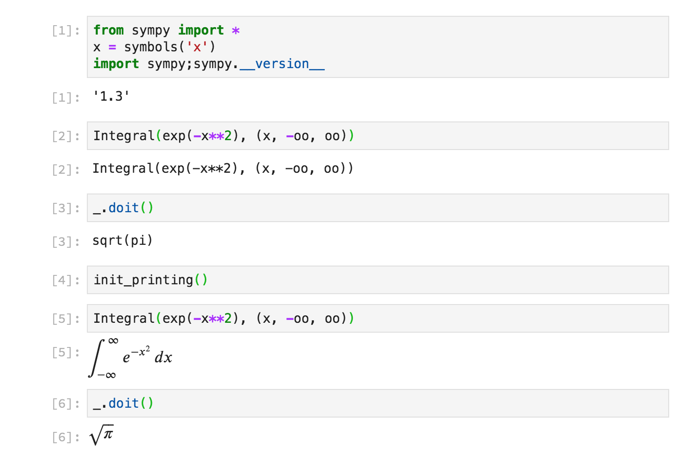
from sympy import *
This will import every public name from the sympy module into the current
namespace. This is often useful because it saves on typing every name that is
used in the import line. This is especially useful when working interactively,
where you just want to import every name and minimize typing.
However, doing from module import * is generally frowned upon in Python. It is
considered acceptable when working interactively at a python prompt, or in
__init__.py files (removestar skips __init__.py files by default).
Some reasons why import * is bad:
- It hides which names are actually imported.
- It is difficult both for human readers and static analyzers such as
pyflakes to tell where a given name comes from when
import *is used. For example, pyflakes cannot detect unused names (for instance, from typos) in the presence ofimport *. - If there are multiple
import *statements, it may not be clear which names come from which module. In some cases, both modules may have a given name, but only the second import will end up being used. This can break people's intuition that the order of imports in a Python file generally does not matter. -
import *often imports more names than you would expect. Unless the module you import defines__all__or carefullydels unused names at the module level,import *will import every public (doesn't start with an underscore) name defined in the module file. This can often include things like standard library imports or loop variables defined at the top-level of the file. For imports from modules (from__init__.py),from module import *will include every submodule defined in that module. Using__all__in modules and__init__.pyfiles is also good practice, as these things are also often confusing even for interactive use whereimport *is acceptable. - In Python 3,
import *is syntactically not allowed inside of a function definition.
Here are some official Python references stating not to use import * in
files:
-
In general, don’t use
from modulename import *. Doing so clutters the importer’s namespace, and makes it much harder for linters to detect undefined names. -
PEP 8 (the official Python style guide):
Wildcard imports (
from <module> import *) should be avoided, as they make it unclear which names are present in the namespace, confusing both readers and many automated tools.
Unfortunately, if you come across a file in the wild that uses import *, it
can be hard to fix it, because you need to find every name in the file that is
imported from the * and manually add an import for it. Removestar makes this
easy by finding which names come from * imports and replacing the import
lines in the file automatically.
As an example, suppose you have a module mymod like
mymod/
  | __init__.py
  | a.py
  | b.py
with
# mymod/a.py
from .b import *

def func(x):
    return x + y
and
# mymod/b.py
x = 1
y = 2
Then removestar works like:
$ removestar -i mymod/
$ cat mymod/a.py
# mymod/a.py
from .b import y

def func(x):
    return x + y
The -i flag causes it to edit a.py in-place. Without it, it would just
print a diff to the terminal.
For implicit star imports and explicit star imports from the same module,
removestar works statically, making use of
pyflakes. This means none of the code is
actually executed. For external imports, it is not possible to work statically
as external imports may include C extension modules, so in that case, it
imports the names dynamically.
removestar can be installed with pip or conda:
pip install removestar
or if you use conda
conda install -c conda-forge removestar
sphinx-math-dollar
In SymPy, we make heavy use of LaTeX math in our documentation. For example,
in our special functions
documentation,
most special functions are defined using a LaTeX formula, like 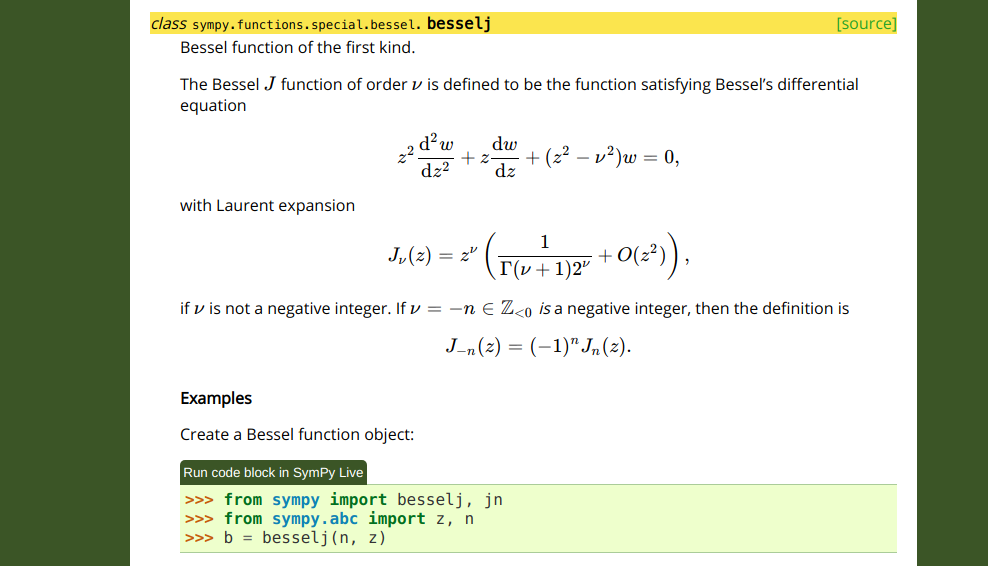
(from https://docs.sympy.org/dev/modules/functions/special.html#sympy.functions.special.bessel.besselj)
However, the source for this math in the docstring of the function uses RST syntax:
class besselj(BesselBase):
    """
    Bessel function of the first kind.

    The Bessel `J` function of order `\nu` is defined to be the function
    satisfying Bessel's differential equation

    .. math ::
        z^2 \frac{\mathrm{d}^2 w}{\mathrm{d}z^2}
        + z \frac{\mathrm{d}w}{\mathrm{d}z} + (z^2 - \nu^2) w = 0,

    with Laurent expansion

    .. math ::
        J_\nu(z) = z^\nu \left(\frac{1}{\Gamma(\nu + 1) 2^\nu} + O(z^2) \right),

    if :math:`\nu` is not a negative integer. If :math:`\nu=-n \in \mathbb{Z}_{<0}`
    *is* a negative integer, then the definition is

    .. math ::
        J_{-n}(z) = (-1)^n J_n(z).
Furthermore, in SymPy's documentation we have configured it so that text
between `single backticks` is rendered as math. This was originally done for
convenience, as the alternative way is to write :math:`\nu` every
time you want to use inline math. But this has lead to many people being
confused, as they are used to Markdown where `single backticks` produce
code.
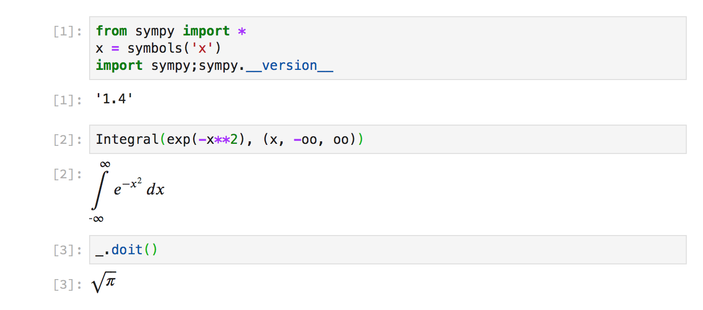
A better way to write this would be if we could delimit math with dollar
signs, like $\nu$. This is how things are done in LaTeX documents, as well
as in things like the Jupyter notebook.
With the new sphinx-math-dollar
Sphinx extension, this is now possible. Writing $\nu$ produces $\nu$, and
the above docstring can now be written as
class besselj(BesselBase):
    """
    Bessel function of the first kind.

    The Bessel $J$ function of order $\nu$ is defined to be the function
    satisfying Bessel's differential equation

    .. math ::
        z^2 \frac{\mathrm{d}^2 w}{\mathrm{d}z^2}
        + z \frac{\mathrm{d}w}{\mathrm{d}z} + (z^2 - \nu^2) w = 0,

    with Laurent expansion

    .. math ::
        J_\nu(z) = z^\nu \left(\frac{1}{\Gamma(\nu + 1) 2^\nu} + O(z^2) \right),

    if $\nu$ is not a negative integer. If $\nu=-n \in \mathbb{Z}_{<0}$
    *is* a negative integer, then the definition is

    .. math ::
        J_{-n}(z) = (-1)^n J_n(z).
We also plan to add support for $$double dollars$$ for display math so that .. math :: is no longer needed either .
For end users, the documentation on docs.sympy.org will continue to render exactly the same, but for developers, it is much easier to read and write.
This extension can be easily used in any Sphinx project. Simply install it with pip or conda:
pip install sphinx-math-dollar
or
conda install -c conda-forge sphinx-math-dollar
Then enable it in your conf.py:
extensions = ['sphinx_math_dollar', 'sphinx.ext.mathjax']
Google Season of Docs
The above work on sphinx-math-dollar is part of work I have been doing to improve the tooling around SymPy's documentation. This has been to assist our technical writer Lauren Glattly, who is working with SymPy for the next three months as part of the new Google Season of Docs program. Lauren's project is to improve the consistency of our docstrings in SymPy. She has already identified many key ways our docstring documentation can be improved, and is currently working on a style guide for writing docstrings. Some of the issues that Lauren has identified require improved tooling around the way the HTML documentation is built to fix. So some other SymPy developers and I have been working on improving this, so that she can focus on the technical writing aspects of our documentation.
Lauren has created a draft style guide for documentation at https://github.com/sympy/sympy/wiki/SymPy-Documentation-Style-Guide. Please take a moment to look at it and if you have any feedback on it, comment below or write to the SymPy mailing list.